The riboFrame Page

The riboFrame (under construction) Page

- Authors: Matteo Ramazzotti*, Luisa Berná, Caludio Donati and Duccio Cavalieri
- Contact: matteo_dot_ramazzotti_at_unifi_dot_it
- Dataset: download
- Program: riboFrame @ GitHub
- Citation: Ramazzotti M et al. Front. Genet., 17 November 2015

* contact for technical details

riboFrame: an improved method for microbial taxonomy profiling from non targeted metagenomics

Introduction

Non targeted metagenomics offers the unprecedented possibility of simultaneously investigate the microbial profile and the genetic capabilities of a sample by a direct analysis of its entire DNA content. The assessment of the microbial taxonomic composition is currently obtained by mapping reads to genomic databases that, although growing, are still limited and biased.
Here we present riboFrame, a novel method for microbial profiling based on the identification and classification of 16S rRNA sequences in non targeted metagenomics datasets. Reads overlapping the 16S rRNA genes are identified using Hidden Markov Models and a taxonomic assignment is obtained by naïve Bayesian classification. All reads identified as ribosomal are coherently positioned in the 16S rRNA gene, allowing the use of the topology of the gene (i.e. the secondary structure and the location of variable regions) to guide the abundance analysis.
We tested and verified the efficacy of our method on simulated ribosomal data, on simulated metagenomes and on a real dataset.
riboFrame exploits the taxonomic potentialities of the 16S rRNA gene in the context of non-targeted metagenomics, giving an accurate perspective on the microbial profile in metagenomic samples.

Program installation

The package riboFrame is composed by two perl scripts, riboTrap.pl and riboMap.pl that can be downloaded from the link above.
A minimal Perl installation is sufficient and needed for the scripts to work.
Two other programs are required, that constitute the working ground of the riboFrame scripts:

Eddy's HMMER3 (hmmer.janelia.org), read more here
RDP's RDPclassifier (rdp.cme.msu.edu), read more here

HMMER3 should be in your distro's repositories and can be easily installed with your package manager. The 2.6 version of RDPclassifier (minimal installation) is shipped with the riboFrame program (download it at the link above) in a zipped format. If you unzip the file, the following files should be created

d: riboFrame
d:   lib
f:      RDPclassifier libraries
d:   hmms
f:      files with bacterial and archeal hmms
f:   riboTrap.pl
f:   riboMap.pl
f:   RDPclassifier.jar
d:   samples

If your setup is ok (and you have HMMER3 installed) we can start learning the basic steps of riboFrame, using the following demo riboFrame analysis.

Demo riboFrame analysis

In order to run the following example, open a linux terminal and go the to the newly created riboFrame folder.

The example that follows runs a full riboFrame analysis on a linux machine and on quality checked Illumina data. The sample come from HMP and can be downloaded and prepared following the commands listed hereinafter. All files but the original .fastq and .fasta generated by the following commands are contained in the dataset file that can be downloaded fom the link above, but if you want to do everything from scratch the following steps must be run:

1. Download QC Illumina reads from HMP with axel (warning, the file is a 6 Gb tar.gz archive!) and extract the tarball

cd sample
axel -n 10 http://downloads.hmpdacc.org/data/Illumina/stool/SRS011061.tar.bz2
tar -xjf SRS011061.tar.bz2
cd ..

2. Extact fasta from fastq. We'll use grep, but feel free to change this step according to your preferences. A third file is present containing singletons. We'll skip it for brevity...

grep -A1 -E "^@.+\/1$" samples/SRS011061.denovo_duplicates_marked.trimmed.1.fastq | grep -v -e "--" | sed 's/^@/>/' > samples/SRS011061.1.fasta
grep -A1 -E "^@.+\/2$" samples/SRS011061.denovo_duplicates_marked.trimmed.2.fastq | grep -v -e "--" | sed 's/^@/>/' > samples/SRS011061.2.fasta
#grep -A1 -E "^@.+\/1$" samples/SRS011061.denovo_duplicates_marked.trimmed.singleton.fastq | grep -v -e "--" | sed 's/^@/>/' >> samples/SRS011061.1.fasta
#grep -A1 -E "^@.+\/2$" samples/SRS011061.denovo_duplicates_marked.trimmed.singleton.fastq | grep -v -e "--" | sed 's/^@/>/' >> samples/SRS011061.2.fasta

3. Catch ribosomal reads with hmmsearch using the HMMs in the provided hmm folder (feel free to change the --cpu option or remove it)

hmmsearch -E 0.00001 --domtblout samples/SRS011061.1.fwd.bact.ribosomal.table --noali --cpu 4 -o /dev/null hmms/16s_bact_for3.hmm samples/SRS011061.1.fasta
hmmsearch -E 0.00001 --domtblout samples/SRS011061.1.rev.bact.ribosomal.table --noali --cpu 4 -o /dev/null hmms/16s_bact_rev3.hmm samples/SRS011061.1.fasta
hmmsearch -E 0.00001 --domtblout samples/SRS011061.1.fwd.arch.ribosomal.table --noali --cpu 4 -o /dev/null hmms/16s_arch_for3.hmm samples/SRS011061.1.fasta
hmmsearch -E 0.00001 --domtblout samples/SRS011061.1.rev.arch.ribosomal.table --noali --cpu 4 -o /dev/null hmms/16s_arch_rev3.hmm samples/SRS011061.1.fasta
hmmsearch -E 0.00001 --domtblout samples/SRS011061.2.fwd.bact.ribosomal.table --noali --cpu 4 -o /dev/null hmms/16s_bact_for3.hmm samples/SRS011061.2.fasta
hmmsearch -E 0.00001 --domtblout samples/SRS011061.2.rev.bact.ribosomal.table --noali --cpu 4 -o /dev/null hmms/16s_bact_rev3.hmm samples/SRS011061.2.fasta
hmmsearch -E 0.00001 --domtblout samples/SRS011061.2.fwd.arch.ribosomal.table --noali --cpu 4 -o /dev/null hmms/16s_arch_for3.hmm samples/SRS011061.2.fasta
hmmsearch -E 0.00001 --domtblout samples/SRS011061.2.rev.arch.ribosomal.table --noali --cpu 4 -o /dev/null hmms/16s_arch_rev3.hmm samples/SRS011061.2.fasta

RiboTrap just use the tabular output of hmmsearch (--domtblout) , so the output "-o" is directed to the null and this output is suppressed.

WARNING: hmmsearch (as BLAST does) stops fasta headers after the first whitespace! riboFrame is compliant with this behavious, so be sure that your fasta headers do not contain whitespaces or at least that reads will stay uniquely identified even after deleting from their headers all characters following the whitespace (included)!!!

4. Use riboTrap to apply 16S rRNA topology to the extracted reads

perl riboTrap.pl samples/SRS011061

The main output of riboTrap is SRS011061.16S.fasta. We'll move on from this. But please note that the option covplot=1 specifies to riboTrap to emit the coverage plot, that is fundamental to understand wether sufficient sampling of the metagenomic dataset is done (i.e. if a sufficient number of ribosomal reads have been extacted) to ensure that abundance will not be biased. To have the covplot plotted, the R software must be installed on your system. The covplot for out data looks like this: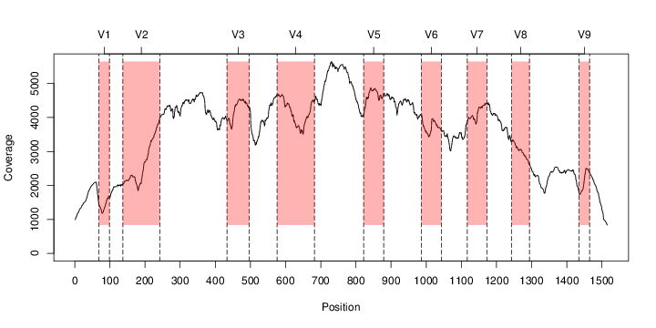

5. Classify 16S reads using RDPclassifier

java -Xmx1g -jar rdp_classifier.jar -q samples/SRS011061.16S.fasta -o samples/SRS011061.16S.rdp

RDPclassifier output SRS011061.16S.rdp can eventually be used for abundance analysis with riboMap.

If you have downlaoded the dataset file and uncompressed it, you can start from here.

Let's impose a taxonomy confidence threshold of 0.8 and accumulate counts. The examples below show four different topology-assisted classifications using

all the available reads

perl riboMap.pl file=samples/SRS011061.16S.rdp var=full conf=0.8 cross=over percmin=0.5 covplot=1 outplot=1 out=samples/SRS011061.ab_full

reads falling in all variable regions

perl riboMap.pl file=samples/SRS011061.16S.rdp var=all conf=0.8 cross=over percmin=0.5 tol=10% covplot=1 outplot=1 out=samples/SRS011061.ab_all

reads contained in the V2 and V3 regions with a 10% tolerance

perl riboMap.pl file=samples/SRS011061.16S.rdp var=V2,V3 conf=0.8 cross=over percmin=0.5 tol=10% covplot=1 outplot=1 out=samples/SRS011061.ab_V2,V3

reads mapping from he beginning of the V5 region to the end of the V6 region

perl riboMap.pl file=samples/SRS011061.16S.rdp var=V5-V6 conf=0.8 cross=over percmin=0.5 tol=10% covplot=1 outplot=1 out=samples/SRS011061.ab_V5-V6

In all cases we set riboMap to avoid reporting elements whose abundance percent was lower than 1%.
We also asked the coverage plots and the abundance plots (works only if you have R installed)

Let's first look at the coverage plots for the four examples, that indicate how many reads were selected for the abundance analysis (try to guess which covplot comes from which example...):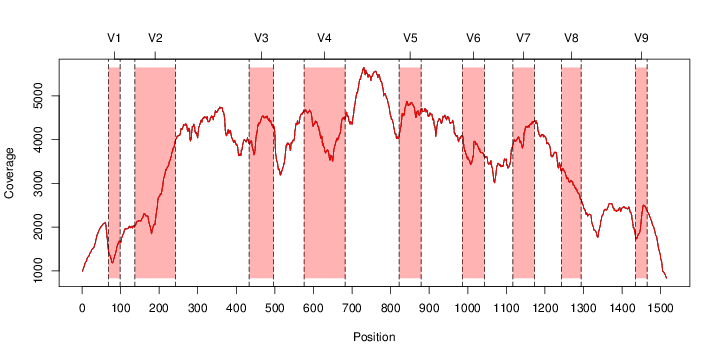

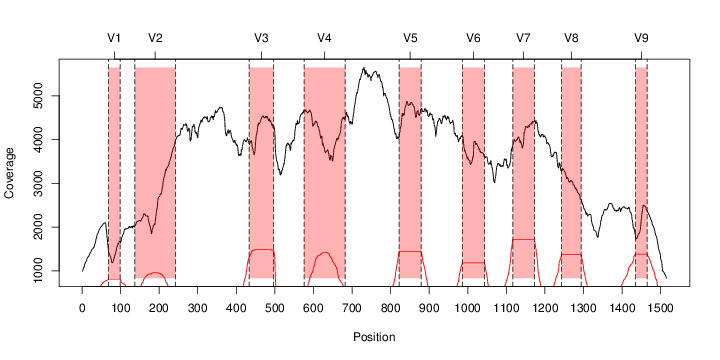
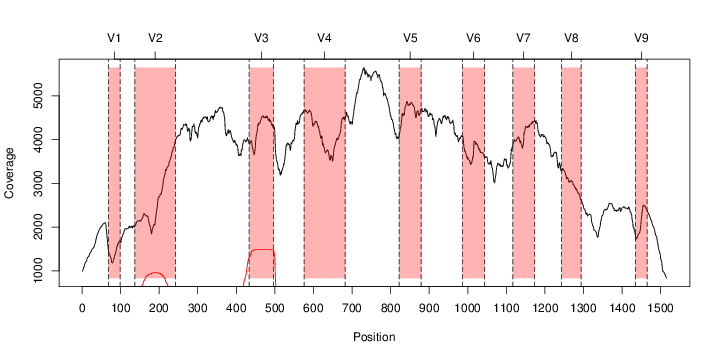
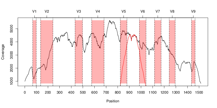
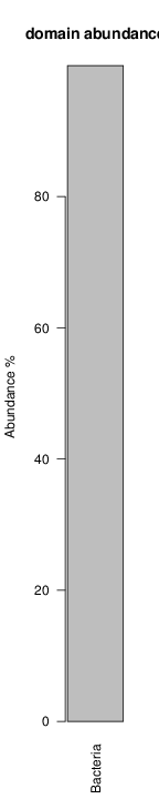
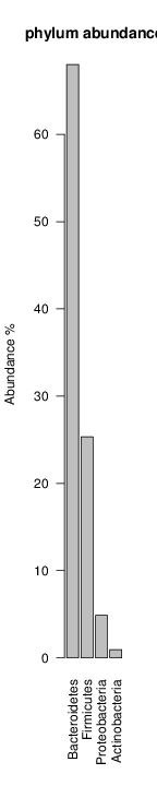
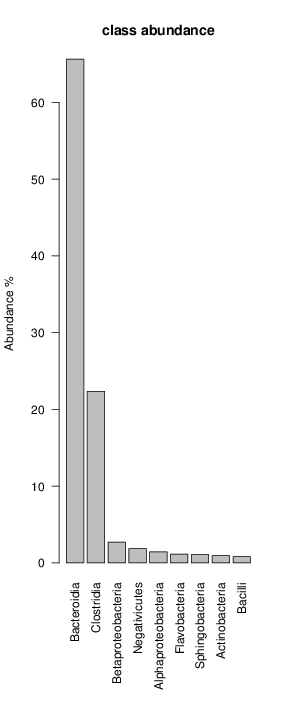
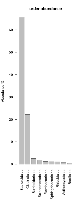
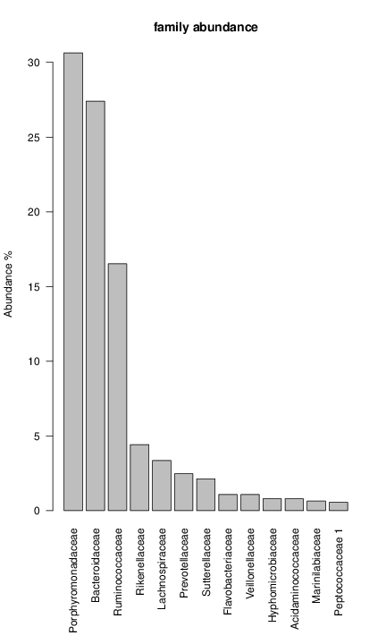
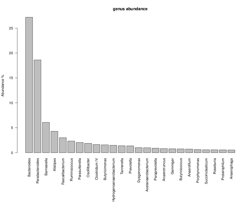
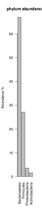
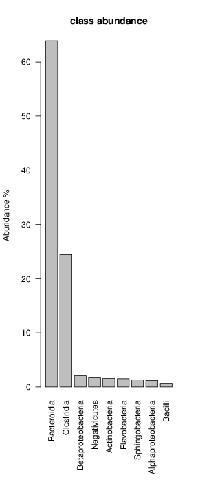
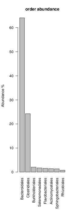
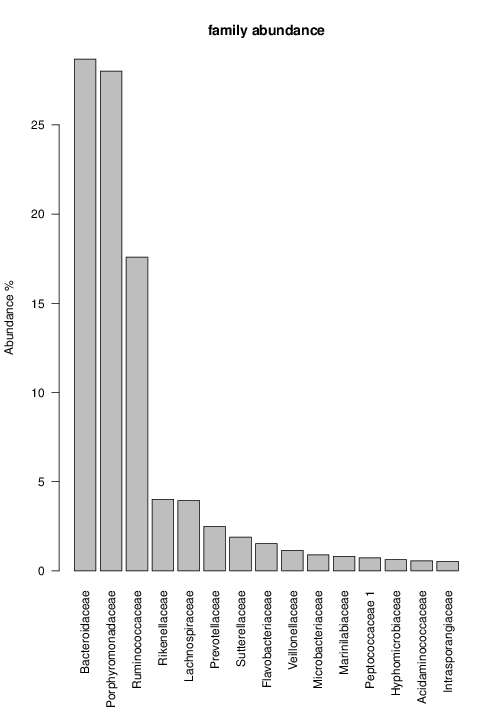
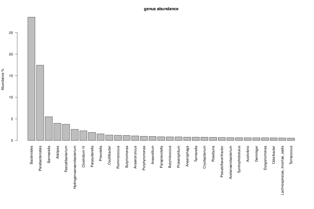
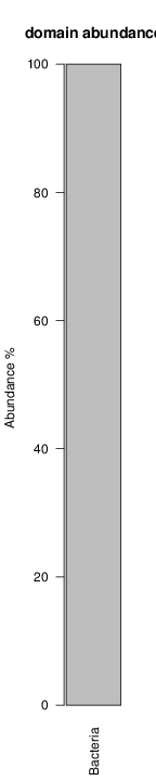
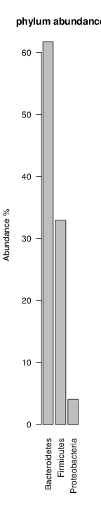
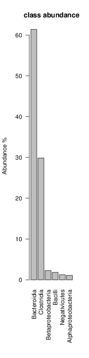
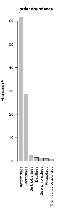
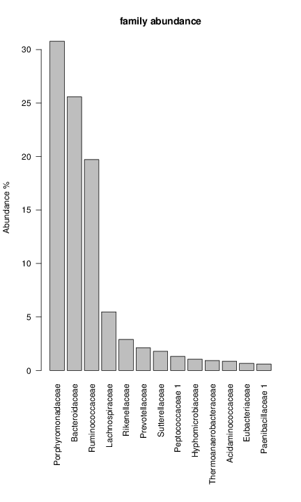
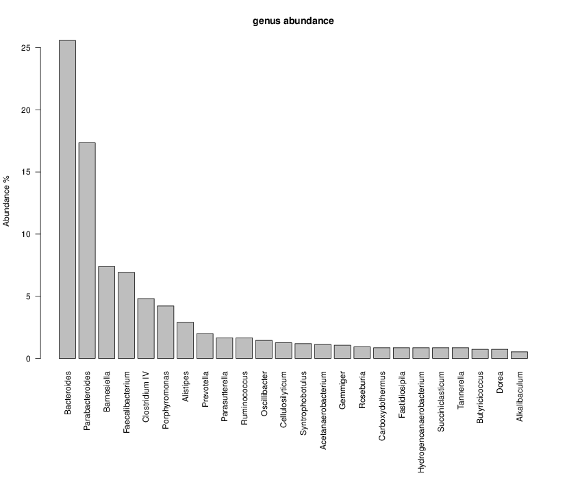
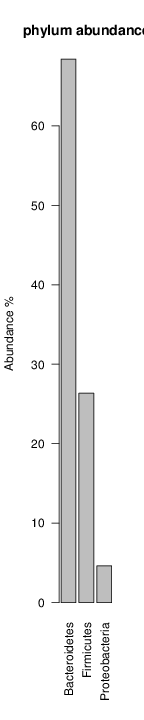
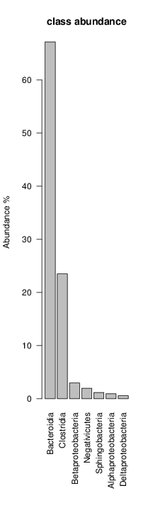
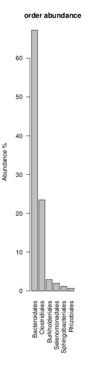
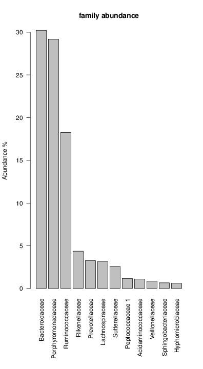
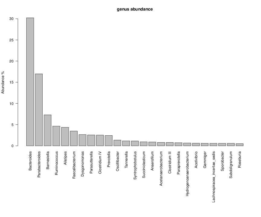
It shoul be clear how the recruitment system works. The black line represents all available reads, the red line represents the selected reads.

Now let's investigate how abundance plots vary in the different analyses:

Example 1. Plots of ranks > 1% with no region selection for reads (var=full)
domain	phylum	class	order	family	genus
Example 2. Plots of ranks > 1% with variable region selection for reads (var=all)
domain	phylum	class	order	family	genus
Example 3. Plots of ranks > 1% using only reads mapping in the V2 OR V3 regions, with 10% length tolerance (var=V2,V3 tol=10%)
domain	phylum	class	order	family	genus
Example 4. Plots of ranks > 1% using only reads mapping from the beginning of the V5 region to the end of the V6 region, with 10% length tolerance (var=V5-V6 tol=10%)
domain	phylum	class	order	family	genus

In the end, ask riboMap how to investigate specific regions

perl riboMap.pl var

A bash script have been created to run the example above. Feel free to download it here

riboTrap outputs explained

riboTrap script emits two types of output files

.fasta: for each run of a sample XXX, three fasta files are written, namely XXX.16S.fasta, XXX.arch.16S.fasta and XXX.bact.16S.fasta.
The .bact.16S and the .arch.16S files contain reads specifically assigned to bacteria and archea, respectively.
The .16S file is a combination of the two and it shoud be used for taxonomic classification.
The header of the fasta format is taken from source reads and the read length and the mapping position on the 16S gene is added. Something like this:
```
>61NLYAAXX100508:6:109:10872:17888:101:225.325
---------------------------------- LLL SSS.EEE

-: original read name
L: read length
SSS: start position
EEE: end position
```
.cov: for each run of a sample XXX, three coverage files are written detailing the coverage on the 16S genes of the archeal, bacterial and combined reads. These files contain the 16S position in the first column (pos) and the coverage in next columns (cnt). It can be used to evaluate how reads of your dataset covers the 16S gene, e.g by producing plots like this:

Appendix

Obtaining raw data from Human Microbiome Project (HMP)
Browse the page http://www.hmpdacc.org/HMASM/ searching for a sample of interest in the data table. Download the reads data from the Reads column (they are > 5Gb files, so we suggest to use the Mozilla DownThemall plugin (that support pause/resume) or the axel downloader for parallel download).